36. The Design and Price of Information#
36.1. Overview#
Earlier lectures in this section asked which statistical experiment a decision maker should prefer.
Blackwell’s Theorem on Comparing Experiments gave the classic answer: experiment \(\mu\) is at least as informative as experiment \(\nu\) when every Bayesian decision maker attains weakly higher expected utility with \(\mu\).
This lecture asks a different question.
Suppose somebody owns the data and wants to sell it.
What should she sell, and at what price?
We study Bergemann et al. [2018], who analyze a monopolist data seller facing a buyer who already has some private information of his own.
The buyer’s private information is exactly what he would like to hide, because it determines his willingness to pay.
So the seller screens by offering a menu of statistical experiments, degrading the information sold to some buyers in order to charge more to others.
The central finding is that degrading information is not simply a matter of adding noise.
Blackwell’s order is a partial order, so two experiments can be ranked differently by different decision makers.
The seller exploits precisely those incomparable pairs: information has a vertical dimension, its quality, and a horizontal dimension, its position.
That horizontal dimension has no counterpart in ordinary monopoly screening over quality or quantity, and it is what allows the seller to extract rents that would otherwise be impossible to reach.
Along the way we will
compute the value of an arbitrary experiment to an arbitrary belief type,
verify numerically that Blackwell’s order fails to rank the experiments the seller wants to use,
solve the two-type screening problem by brute force and check it against the paper’s closed forms,
solve the continuum-of-types problem as a linear program, which reproduces the paper’s ironing and pooling results without any need to implement ironing by hand.
Let’s start with imports.
import matplotlib.pyplot as plt
import numpy as np
from scipy import stats
from scipy.optimize import linprog

plt.rcParams['figure.figsize'] = (10, 5)
np.set_printoptions(precision=4, suppress=True)
36.2. The decision problem#
A data buyer must choose an action \(a\) from a finite set \(A\) without knowing the state \(\omega\), which lives in a finite set \(\Omega\).
We work throughout with the matching case in which the buyer wants his action to match the state,
so that matching state \(\omega_i\) pays \(u_i > 0\) and any mismatch pays zero.
From here on we take two states and two actions, \(\Omega = \{\omega_1, \omega_2\}\) and \(A = \{a_1, a_2\}\), which is the case Bergemann et al. [2018] solve completely.
The buyer’s type is his interim belief
which is private information.
The seller knows only the distribution \(F\) from which \(\theta\) is drawn.
Without extra information the buyer picks the better of two constant actions, so his reservation utility is
The type that is least sure what to do is the one where the two terms are equal,
Types above \(\theta^*\) would choose \(a_1\) on their own, types below would choose \(a_2\).
Note
The buyer’s belief \(\theta\) can be generated from a common prior together with a privately observed signal, exactly as in Likelihood Ratio Processes and Bayesian Learning.
A buyer with a very precise private signal has \(\theta\) near \(0\) or \(1\); a buyer who has learned nothing sits near \(\theta^*\).
So “high type” in this lecture means badly informed, and it is the badly informed buyer who is willing to pay the most.
36.3. Experiments and their value#
A statistical experiment is a stochastic matrix mapping states into signals.
With two states and two actions it suffices to consider two signals, and we write
where row \(i\) gives the signal distribution in state \(\omega_i\).
Thus \(\pi_1 = \Pr[s_1 \mid \omega_1]\) and \(\pi_2 = \Pr[s_2 \mid \omega_2]\).
We adopt the normalization \(\pi_1 + \pi_2 \geq 1\), which just says that signal \(s_1\) is relatively more likely in state \(\omega_1\) than in state \(\omega_2\).
The fully informative experiment \(\overline{E}\) has \(\pi_1 = \pi_2 = 1\).
After seeing signal \(s_k\) the buyer picks the action with the highest expected payoff, so his gross value is obtained by summing the best he can do signal by signal.
Subtracting his reservation utility (36.2) gives the net value of information
def value(pi1, pi2, theta, u1=1.0, u2=1.0):
    """Net value of experiment (pi1, pi2) to a buyer with belief theta."""
    theta = np.asarray(theta, dtype=float)
    s1 = np.maximum(theta * pi1 * u1, (1 - theta) * (1 - pi2) * u2)
    s2 = np.maximum(theta * (1 - pi1) * u1, (1 - theta) * pi2 * u2)
    return s1 + s2 - np.maximum(theta * u1, (1 - theta) * u2)
If the buyer simply obeys the recommendation implicit in each signal, taking \(a_1\) after \(s_1\) and \(a_2\) after \(s_2\), the value collapses to
which is the expression the paper works with.
def value_obedient(pi1, pi2, theta, u1=1.0, u2=1.0):
    """Value when the buyer follows the recommendation, or ignores the signal."""
    theta = np.asarray(theta, dtype=float)
    return np.maximum(theta * pi1 * u1 + (1 - theta) * pi2 * u2
                      - np.maximum(theta * u1, (1 - theta) * u2), 0.0)
The two expressions agree exactly under the normalization \(\pi_1 + \pi_2 \geq 1\) and can differ sharply without it, which is what the normalization is for.
grid = np.linspace(0, 1, 2001)
worst_ok = worst_bad = 0.0
for p1 in np.linspace(0, 1, 51):
    for p2 in np.linspace(0, 1, 51):
        gap = np.abs(value(p1, p2, grid) - value_obedient(p1, p2, grid)).max()
        if p1 + p2 >= 1:
            worst_ok = max(worst_ok, gap)
        else:
            worst_bad = max(worst_bad, gap)

print(f'largest gap where pi1 + pi2 >= 1:  {worst_ok:.2e}')
print(f'largest gap where pi1 + pi2 <  1:  {worst_bad:.4f}')
largest gap where pi1 + pi2 >= 1:  1.11e-16
largest gap where pi1 + pi2 <  1:  0.5000
We use the general form (36.5) from here on, since a buyer who misreports his type will not in general want to obey the recommendations built into somebody else’s experiment.
Here is the value of information as a function of the buyer’s type.
theta = np.linspace(0, 1, 1001)

fig, axes = plt.subplots(1, 2, figsize=(11, 4))
for ax, (p1, p2), ttl in zip(
        axes, [(1.0, 1.0), (0.5, 1.0)],
        [r'fully informative $(\pi_1,\pi_2)=(1,1)$',
         r'partially informative $(\pi_1,\pi_2)=(1/2,1)$']):
    ax.plot(theta, value(p1, p2, theta), lw=2)
    ax.axvline(0.5, color='0.6', ls='--', lw=1)
    ax.set(xlabel=r'$\theta$', ylabel=r'$V(E,\theta)$', title=ttl)
fig.suptitle('Value of information, $u_1 = u_2 = 1$')
fig.tight_layout()
plt.show()
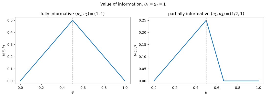
Fig. 36.1 Value of full and partial information#
Three features of these pictures drive everything that follows.
The value is piecewise linear in \(\theta\), because types are probabilities and expected utilities are linear in probabilities.
The value is highest at \(\theta^*\) and falls to zero at \(\theta \in \{0, 1\}\): the buyer who already knows the state will pay nothing, and the buyer who knows least will pay most.
The partially informative experiment in the right panel is worth nothing at all to types above \(2/3\), even though it is worth a great deal to types just below \(1/2\).
That last property is the seller’s main tool.
36.4. Blackwell’s order is only partial#
Blackwell’s Theorem on Comparing Experiments establishes that experiment \(E\) is at least as informative as \(E'\) in Blackwell’s sense exactly when \(E'\) is a garbling of \(E\), meaning there is a stochastic matrix \(M\) with
When \(E\) is invertible this is easy to check: solve \(M = E^{-1}E'\) and ask whether \(M\) is a stochastic matrix.
def experiment(pi1, pi2):
    return np.array([[pi1, 1 - pi1], [1 - pi2, pi2]])


def garbling(E, Ep, tol=1e-9):
    """Return M with Ep = E @ M if Ep is a garbling of E, else None."""
    if abs(np.linalg.det(E)) < tol:
        return None
    M = np.linalg.solve(E, Ep)
    if (M > -tol).all() and np.allclose(M.sum(axis=1), 1, atol=tol):
        return M
    return None


pairs = [((1, 1), (0.8, 1)), ((1, 1), (1, 0.8)),
         ((0.9, 0.9), (0.8, 0.8)),
         ((0.8, 1), (1, 0.8)), ((1, 0.8), (0.8, 1))]
for a, b in pairs:
    ok = garbling(experiment(*a), experiment(*b)) is not None
    print(f'  is {b} a garbling of {a}?  {"yes" if ok else "no"}')
  is (0.8, 1) a garbling of (1, 1)?  yes
  is (1, 0.8) a garbling of (1, 1)?  yes
  is (0.8, 0.8) a garbling of (0.9, 0.9)?  yes
  is (1, 0.8) a garbling of (0.8, 1)?  no
  is (0.8, 1) a garbling of (1, 0.8)?  no
The fully informative experiment garbles into everything, and \((0.9, 0.9)\) garbles into the uniformly noisier \((0.8, 0.8)\).
Those are the vertical comparisons, and Blackwell’s theorem says every type agrees about them.
But \((0.8, 1)\) and \((1, 0.8)\) garble into each other in neither direction.
Blackwell’s order simply does not rank them, and that means different types are free to rank them differently.
va, vb = value(0.8, 1, theta), value(1, 0.8, theta)

fig, ax = plt.subplots()
ax.plot(theta, va, lw=2, label=r'$E_a = (0.8, 1)$')
ax.plot(theta, vb, lw=2, label=r'$E_b = (1, 0.8)$')
ax.fill_between(theta, va, vb, where=va > vb, alpha=0.15, color='C0')
ax.fill_between(theta, va, vb, where=vb > va, alpha=0.15, color='C1')
ax.axvline(0.5, color='0.4', ls='--', lw=1)
ax.set(xlabel=r'$\theta$', ylabel=r'$V(E,\theta)$',
       title='Types below $1/2$ prefer $E_a$, types above prefer $E_b$')
ax.legend()
fig.tight_layout()
plt.show()

for t in [0.2, 0.35, 0.65, 0.8]:
    pref = 'E_a' if value(0.8, 1, t) > value(1, 0.8, t) else 'E_b'
    print(f'  theta = {t}:  V(E_a) = {value(0.8, 1, t):.4f},'
          f'  V(E_b) = {value(1, 0.8, t):.4f}   prefers {pref}')
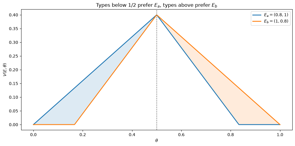
Fig. 36.2 Two experiments that Blackwell’s order does not rank#
  theta = 0.2:  V(E_a) = 0.1600,  V(E_b) = 0.0400   prefers E_a
  theta = 0.35:  V(E_a) = 0.2800,  V(E_b) = 0.2200   prefers E_a
  theta = 0.65:  V(E_a) = 0.2200,  V(E_b) = 0.2800   prefers E_b
  theta = 0.8:  V(E_a) = 0.0400,  V(E_b) = 0.1600   prefers E_b
\(E_a\) is better at ruling out state \(\omega_2\) and \(E_b\) is better at ruling out state \(\omega_1\).
A buyer who already thinks \(\omega_1\) is likely wants help distinguishing among the possibilities he has not ruled out, so he values \(E_b\); a buyer who leans the other way values \(E_a\).
This is the horizontal dimension of information.
In ordinary nonlinear pricing over quality or quantity, all types agree on the ranking of products and the seller can only move up and down a single ladder.
Here the seller has a second dial, and turning it lets her hand one type something that is worthless to another.
36.5. The seller’s problem#
The seller commits to a menu \(\{E(\theta), t(\theta)\}\) assigning an experiment and a price to each reported type.
Payments cannot be made contingent on the state, the signal, or the buyer’s action, so the value of an experiment to a buyer is determined by his belief alone.
Writing \(V(\theta) = V(E(\theta), \theta) - t(\theta)\) for the buyer’s rent, the seller solves
subject to incentive compatibility and individual rationality,
Bergemann et al. [2018] establish two structural results that we will see confirmed in every menu we compute.
Proposition 36.1
In any optimal menu:
the fully informative experiment \(\overline{E}\) is offered;
every experiment is nondispersed, meaning \(\pi_{ij} = 0\) for some \(i \neq j\);
in the matching case every experiment is concentrated, meaning \(\pi_{ii} = 1\) for some \(i\).
Part 3 says that in our binary setting every experiment on the menu has \(\pi_1 = 1\) or \(\pi_2 = 1\).
Optimal degradation never adds unbiased noise everywhere; it leaves one state perfectly detectable and blurs the other.
36.6. Two types#
Take two types \(\theta^L\) and \(\theta^H\), with \(\theta^H\) the high value type in the sense that he values the fully informative experiment more,
With \(u_1 = u_2\) this says \(|\theta^H - 1/2| \leq |\theta^L - 1/2|\), so the high type is the one who is less well informed to begin with.
Let \(\gamma = \Pr[\theta = \theta^H]\).
The types are congruent if \(\theta^* < \theta^H < \theta^L\), so both would take the same action without extra information, and noncongruent if \(\theta^L < \theta^* < \theta^H\).
An optimal menu has the familiar shape: the high type buys \(\overline{E}\), the low type’s participation constraint binds, and the high type’s incentive constraint binds.
Those three facts pin down both prices once the low type’s experiment is chosen.
def two_type_revenue(pi1, pi2, tL, tH, gamma, u1=1.0, u2=1.0):
    """Revenue when the high type buys E_bar and the low type buys (pi1, pi2)."""
    VbarH, VbarL = value(1, 1, tH, u1, u2), value(1, 1, tL, u1, u2)
    VL_L, VL_H = value(pi1, pi2, tL, u1, u2), value(pi1, pi2, tH, u1, u2)
    t_low = VL_L                                  # low type's IR binds
    t_high = VbarH - VL_H + t_low                 # high type's IC binds
    if t_high > VbarH + 1e-12:                    # high type must participate
        return -np.inf
    if VbarL - t_high > 1e-12:                    # low type must not deviate
        return -np.inf
    return gamma * t_high + (1 - gamma) * t_low
36.6.1. Noncongruent types#
Set \(\theta^L = 1/5\) and \(\theta^H = 7/10\) with \(u_1 = u_2 = 1\), so that \(\theta^* = 1/2\) lies between them.
Because the two types would take different actions on their own, the seller can build an experiment that is valuable to one and worthless to the other.
Choosing \(\pi_2 = 1\) and
leaves the high type exactly indifferent between his two actions after signal \(s_1\), so the experiment is worth nothing to him while the low type values it strictly.
That is feasible but not optimal.
The seller does better by making the high type’s incentive constraint bind instead, which gives
tL, tH, u1, u2 = 0.2, 0.7, 1.0, 1.0
pi1_zero = (u1 * tH - u2 * (1 - tH)) / (u1 * tH)
pi1_opt = (u1 * tH - u2 * (1 - tH)) / (u1 * (tH - tL))

print(f'zero-value-to-high experiment   pi1 = {pi1_zero:.4f}  (= 4/7)')
print(f'binding-IC experiment           pi1 = {pi1_opt:.4f}  (= 4/5)')
print(f'\n  V(E_zero, theta_H) = {value(pi1_zero, 1, tH):.4f}')
print(f'  V(E_opt,  theta_L) = {value(pi1_opt, 1, tL):.4f}'
      f'    V(E_opt, theta_H) = {value(pi1_opt, 1, tH):.4f}')
zero-value-to-high experiment   pi1 = 0.5714  (= 4/7)
binding-IC experiment           pi1 = 0.8000  (= 4/5)

  V(E_zero, theta_H) = 0.0000
  V(E_opt,  theta_L) = 0.1600    V(E_opt, theta_H) = 0.1600
The second experiment gives both types the same gross value, so the seller can charge each of them exactly what the information is worth and leave no rent at all.
fig, axes = plt.subplots(1, 2, figsize=(12, 4.2))
for ax, p1, ttl in zip(axes, [pi1_zero, pi1_opt],
                       ['suboptimal menu: partial experiment worth zero to $\\theta^H$',
                        'optimal menu: high type indifferent between the two items']):
    t_hi = value(1, 1, tH)                                     # price of E_bar
    t_lo = value(p1, 1, tL)                                    # price of partial item
    ax.plot(theta, value(1, 1, theta) - t_hi, lw=2, label='fully informative')
    ax.plot(theta, value(p1, 1, theta) - t_lo, lw=2, ls='--',
            label=f'partial, $\\pi_1={p1:.3f}$')
    ax.axhline(0, color='0.3', lw=1)
    for t, nm in [(tL, r'$\theta^L$'), (tH, r'$\theta^H$')]:
        ax.axvline(t, color='0.7', ls=':', lw=1)
        ax.annotate(nm, (t, ax.get_ylim()[0]), fontsize=9)
    ax.set(xlabel=r'$\theta$', ylabel=r'$V - t$', title=ttl, ylim=(-0.35, 0.25))
    ax.legend(fontsize=8, loc='upper left')
fig.tight_layout()
plt.show()
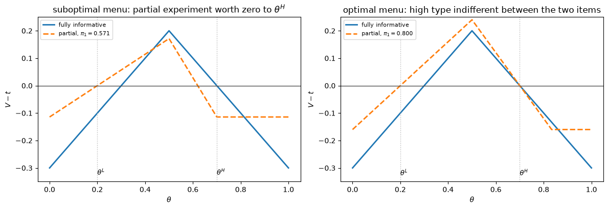
Fig. 36.3 Net value of the two menus as a function of the buyer’s type#
In the left panel the high type’s net value of the fully informative experiment lies strictly above his net value of the partial one, so his incentive constraint is slack and the seller is leaving money on the table.
In the right panel the two curves meet exactly at \(\theta^H\).
Now we check the closed form (36.11) against a brute-force search over all experiments.
def brute_force(tL, tH, gamma, n=301, u1=1.0, u2=1.0):
    """Search over all (pi1, pi2) for the best low-type experiment."""
    g = np.linspace(0, 1, n)
    best, arg = -np.inf, None
    for p1 in g:
        for p2 in g:
            if p1 + p2 < 1:
                continue
            r = two_type_revenue(p1, p2, tL, tH, gamma, u1, u2)
            if r > best:
                best, arg = r, (p1, p2)
    return best, arg


print(f'{"gamma":>7s}{"brute force":>13s}{"argmax":>18s}'
      f'{"eq (20) menu":>14s}{"E_bar to both":>15s}')
for gamma in [0.10, 0.25, 0.30, 0.50, 0.90]:
    best, arg = brute_force(tL, tH, gamma)
    closed = two_type_revenue(pi1_opt, 1.0, tL, tH, gamma)
    both = two_type_revenue(1.0, 1.0, tL, tH, gamma)
    print(f'{gamma:7.2f}{best:13.5f}   ({arg[0]:.3f}, {arg[1]:.3f})'
          f'{closed:14.5f}{both:15.5f}')
print(f'\nthe paper: discriminate iff gamma > theta_L / theta_H = {tL / tH:.4f}')
  gamma  brute force            argmax  eq (20) menu  E_bar to both
   0.10      0.20000   (1.000, 1.000)       0.17400        0.20000
   0.25      0.20000   (1.000, 1.000)       0.19500        0.20000
   0.30      0.20200   (0.800, 1.000)       0.20200        0.20000
   0.50      0.23000   (0.800, 1.000)       0.23000        0.20000
   0.90      0.28600   (0.800, 1.000)       0.28600        0.20000

the paper: discriminate iff gamma > theta_L / theta_H = 0.2857
The brute-force optimum sits at \((\pi_1, \pi_2) = (0.8, 1)\) whenever discrimination pays, matching (36.11) exactly, and at \((1, 1)\) otherwise.
The switch happens right at \(\gamma = \theta^L / \theta^H\).
When low types are common the seller prefers to sell everyone the fully informative experiment cheaply; when high types are common she prefers to protect the high price by degrading what the low type gets.
Note also that both experiments in the optimal menu have \(\pi_2 = 1\), confirming part 3 of Proposition 36.1.
36.7. A continuum of types#
Now let \(\theta\) be distributed on \([0,1]\) with density \(f\) and distribution \(F\).
The key simplification is that the value of an experiment depends on \((\pi_1, \pi_2)\) only through the scalar
which Bergemann et al. [2018] call the differential informativeness of the experiment.
In terms of \(q\) the value becomes
The fully informative experiment is \(q = u_1 - u_2\).
The two endpoints \(q = -u_2\) and \(q = u_1\) are the experiments in which one signal occurs with probability one in both states, so they convey nothing.
def value_q(q, theta, u1=1.0, u2=1.0):
    """Value of the experiment with differential informativeness q."""
    theta = np.asarray(theta, dtype=float)
    gross = theta * q + u2 + np.minimum(u1 - u2 - q, 0.0)
    return np.maximum(gross - np.maximum(theta * u1, (1 - theta) * u2), 0.0)


def q_to_experiment(q, u1=1.0, u2=1.0):
    """Recover (pi1, pi2) from q using pi1 = 1 or pi2 = 1."""
    return (1.0, (u1 - q) / u2) if q >= u1 - u2 else ((q + u2) / u1, 1.0)


for q in [-1.0, -0.5, 0.0, 0.5, 1.0]:
    p1, p2 = q_to_experiment(q)
    print(f'  q = {q:+.2f}  ->  (pi1, pi2) = ({p1:.3f}, {p2:.3f}),'
          f'   max value over types = {value_q(q, theta).max():.4f}')
  q = -1.00  ->  (pi1, pi2) = (0.000, 1.000),   max value over types = 0.0000
  q = -0.50  ->  (pi1, pi2) = (0.500, 1.000),   max value over types = 0.2500
  q = +0.00  ->  (pi1, pi2) = (1.000, 1.000),   max value over types = 0.5000
  q = +0.50  ->  (pi1, pi2) = (1.000, 0.500),   max value over types = 0.2500
  q = +1.00  ->  (pi1, pi2) = (1.000, 0.000),   max value over types = 0.0000
A menu is now a function \(q(\theta)\), and incentive compatibility requires it to be non-decreasing.
Types who think \(\omega_1\) is more likely want experiments with higher \(q\), which deliver sharper evidence about the state they consider less likely.
There is a second, less familiar restriction.
Because information is worthless to types \(\theta \in \{0, 1\}\), applying the envelope theorem separately on \([0, \theta^*]\) and \([\theta^*, 1]\) and matching the two expressions for the rent of the pivotal type \(\theta^*\) forces
Note that this integral is taken with respect to \(d\theta\), not \(dF(\theta)\).
With those two constraints, the seller’s problem reduces to
subject to \(q\) non-decreasing and (36.14).
36.7.1. Solving it as a linear program#
The integrand of (36.15) is concave and piecewise linear in \(q\), since \(\min\{(d - q) f, 0\} = -f \max\{q - d, 0\}\) with \(d = u_1 - u_2\) and \(f \geq 0\).
Maximizing a concave piecewise-linear objective subject to linear constraints is a linear program.
Introducing \(z(\theta) \geq \max\{q(\theta) - d,\ 0\}\) and discretizing \(\theta\) on a grid gives
subject to \(z_n \geq q_n - d\), \(z_n \geq 0\), \(q_{n+1} \geq q_n\), \(-u_2 \leq q_n \leq u_1\), and \(\sum_n w_n q_n = d\).
def solve_menu(theta, f, u1=1.0, u2=1.0):
    """Solve the seller's problem on a grid of types by linear programming."""
    N = len(theta)
    dth = theta[1] - theta[0]
    F = np.cumsum(f) * dth
    F = F / F[-1]
    w = np.full(N, dth)
    d = u1 - u2

    c = np.concatenate([-(theta * f + F) * w, f * w])       # linprog minimizes
    A_ub = np.hstack([np.eye(N), -np.eye(N)])               # q - z <= d
    b_ub = np.full(N, d)
    D = np.zeros((N - 1, 2 * N))                            # q_n - q_{n+1} <= 0
    rows = np.arange(N - 1)
    D[rows, rows], D[rows, rows + 1] = 1.0, -1.0
    A_ub = np.vstack([A_ub, D])
    b_ub = np.concatenate([b_ub, np.zeros(N - 1)])
    A_eq = np.concatenate([w, np.zeros(N)])[None, :]        # integral constraint
    bounds = [(-u2, u1)] * N + [(0, None)] * N

    res = linprog(c, A_ub=A_ub, b_ub=b_ub, A_eq=A_eq, b_eq=np.array([d]),
                  bounds=bounds, method='highs')
    return res.x[:N], res
The linear program handles the monotonicity constraint automatically.
This matters, because the alternative is to implement Myerson’s ironing procedure by hand: form the virtual values
replace them by the derivatives of the convex hulls of their integrals, and then find the multiplier on (36.14) (see Myerson [1981] and Toikka [2011]).
The linear program does all of that implicitly.
We also want the prices, which follow from the requirement that a buyer at the boundary between two items be indifferent between them.
def menu_items(theta, q, u1=1.0, u2=1.0, tol=1e-4, min_width=0.01):
    """Distinct items in the menu, with the interval of types served and the price.

    Values of q taken on a negligible set of types are transition artifacts of the
    grid, not items on the menu, so we drop them.
    """
    qr = np.round(q / tol) * tol
    vals = [v for v in np.unique(qr)
            if theta[qr == v].max() - theta[qr == v].min() >= min_width]
    items = sorted([(v, theta[qr == v].min(), theta[qr == v].max()) for v in vals],
                   key=lambda x: x[1])
    out, prev_v, prev_t = [], None, 0.0
    for v, lo, hi in items:
        if value_q(v, theta, u1, u2).max() < 1e-9:      # uninformative item
            price = 0.0
        elif prev_v is None:
            price = 0.0
        else:
            price = float(value_q(v, lo, u1, u2)
                          - value_q(prev_v, lo, u1, u2) + prev_t)
        out.append((v, lo, hi, price))
        prev_v, prev_t = v, price
    return out
36.7.2. Uniformly distributed types#
With \(u_1 = u_2 = 1\) and \(\theta\) uniform, the virtual values are \(\phi^-(\theta) = 2\theta\) and \(\phi^+(\theta) = 2\theta - 1\).
Both are strictly increasing, so no ironing is required and the optimal menu should contain a single informative item.
N = 2001
theta_g = np.linspace(0, 1, N)
q_unif, res = solve_menu(theta_g, np.ones(N))

print('LP status:', res.message)
print('distinct values of q:', np.unique(np.round(q_unif, 4)))
for v, lo, hi, p in menu_items(theta_g, q_unif):
    p1, p2 = q_to_experiment(v)
    print(f'   q = {v:+.4f}  (pi1, pi2) = ({p1:.3f}, {p2:.3f})'
          f'   types [{lo:.3f}, {hi:.3f}]   price {p:.4f}')
LP status: Optimization terminated successfully. (HiGHS Status 7: Optimal)
distinct values of q: [-1. -0.  1.]
   q = -1.0000  (pi1, pi2) = (0.000, 1.000)   types [0.000, 0.249]   price 0.0000
   q = -0.0000  (pi1, pi2) = (1.000, 1.000)   types [0.250, 0.750]   price 0.2500
   q = +1.0000  (pi1, pi2) = (1.000, 0.000)   types [0.751, 1.000]   price 0.0000
The seller offers the fully informative experiment to the middle range of types at a single price and nothing to anyone else.
The cutoffs and the price match the analytic solution of Bergemann et al. [2018] exactly: full information to \(\theta \in [1/4, 3/4]\) at a price of \(1/4\).
This is the “no-haggling” outcome of Riley and Zeckhauser [1983] adapted to information.
fig, axes = plt.subplots(1, 2, figsize=(12, 4))
axes[0].plot(theta_g, 2 * theta_g, lw=2, label=r'$\phi^-(\theta) = 2\theta$')
axes[0].plot(theta_g, 2 * theta_g - 1, lw=2, label=r'$\phi^+(\theta) = 2\theta - 1$')
axes[0].axhline(0.5, color='0.4', ls='--', lw=1, label=r'$\lambda^* = 1/2$')
axes[0].set(xlabel=r'$\theta$', title='virtual values, both strictly increasing')
axes[0].legend(fontsize=9)

axes[1].step(theta_g, q_unif, lw=2, where='mid')
axes[1].set(xlabel=r'$\theta$', ylabel=r'$q^*(\theta)$', ylim=(-1.15, 1.15),
            title='optimal menu: one informative item')
axes[1].annotate('no information', (0.06, -0.85), fontsize=9)
axes[1].annotate('full information', (0.38, 0.12), fontsize=9)
axes[1].annotate('no information', (0.78, 0.85), fontsize=9)
fig.tight_layout()
plt.show()
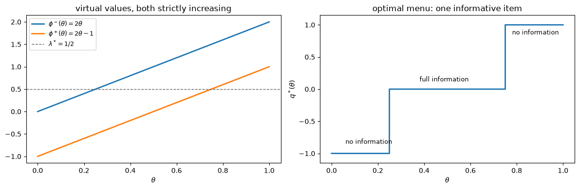
Fig. 36.4 Optimal menu with uniformly distributed types#
36.7.3. Bimodal types and the case for versioning#
Corollary 1 of Bergemann et al. [2018] says that a second experiment is offered only when the virtual values require ironing.
Since types are beliefs, a natural way to break regularity is a population in which most buyers are already well informed, so that the density piles up near both ends.
We follow the paper and take an equal mixture of \(\text{Beta}(8, 30)\) and \(\text{Beta}(60, 30)\).
f_bimodal = (0.5 * stats.beta(8, 30).pdf(theta_g)
             + 0.5 * stats.beta(60, 30).pdf(theta_g))
q_bi, res_bi = solve_menu(theta_g, f_bimodal)

print('LP status:', res_bi.message)
print('distinct values of q:', np.unique(np.round(q_bi, 3)))
print()
for v, lo, hi, p in menu_items(theta_g, q_bi):
    p1, p2 = q_to_experiment(v)
    label = 'no information' if abs(p) < 1e-9 else (
        'full information' if abs(v) < 1e-6 else 'partial information')
    print(f'   q = {v:+.4f}  (pi1, pi2) = ({p1:.3f}, {p2:.3f})'
          f'   types [{lo:.3f}, {hi:.3f}]   price {p:.4f}   {label}')
LP status: Optimization terminated successfully. (HiGHS Status 7: Optimal)
distinct values of q: [-1.    -0.214 -0.     1.   ]

   q = -1.0000  (pi1, pi2) = (0.000, 1.000)   types [0.000, 0.175]   price 0.0000   no information
   q = -0.2141  (pi1, pi2) = (0.786, 1.000)   types [0.175, 0.550]   price 0.1375   partial information
   q = -0.0000  (pi1, pi2) = (1.000, 1.000)   types [0.551, 0.745]   price 0.2555   full information
   q = +1.0000  (pi1, pi2) = (1.000, 0.000)   types [0.745, 1.000]   price 0.0000   no information
Now the menu contains two informative items, in line with Proposition 36.1 and with the result that an optimal menu never contains more than two.
The partial item has \(\pi_2 = 1\), so signal \(s_1\) occurs only in state \(\omega_1\) and perfectly reveals it, while signal \(s_2\) leaves the buyer uncertain.
It is bought by a range of relatively well-informed types who would not pay the price the seller wants to charge the large mass of buyers near \(\theta \approx 0.7\).
items = menu_items(theta_g, q_bi)

fig, axes = plt.subplots(1, 2, figsize=(12, 4))
axes[0].plot(theta_g, f_bimodal, lw=2, color='C2')
axes[0].fill_between(theta_g, f_bimodal, alpha=0.2, color='C2')
axes[0].set(xlabel=r'$\theta$', ylabel='density',
            title='most buyers are already well informed')

axes[1].step(theta_g, q_bi, lw=2, where='mid')
axes[1].set(xlabel=r'$\theta$', ylabel=r'$q^*(\theta)$', ylim=(-1.15, 1.15),
            title='optimal menu: two informative items')
for v, lo, hi, p in items:
    if p > 1e-9:
        axes[1].annotate(f'price {p:.3f}', ((lo + hi) / 2, v + 0.12),
                         ha='center', fontsize=9)
fig.tight_layout()
plt.show()
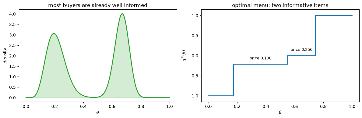
Fig. 36.5 Bimodal type density and the resulting two-item menu#
We can see directly why the seller bothers.
def revenue(theta, q, f, u1=1.0, u2=1.0):
    """Expected revenue from the menu q under density f."""
    dth = theta[1] - theta[0]
    price = np.zeros_like(theta)
    for v, lo, hi, p in menu_items(theta, q, u1, u2):
        price[(theta >= lo) & (theta <= hi)] = p
    return np.sum(price * f) * dth / (np.sum(f) * dth)


q_single = np.where(q_bi < -0.5, -1.0, np.where(q_bi > 0.5, 1.0, 0.0))
print(f'revenue, optimal two-item menu   {revenue(theta_g, q_bi, f_bimodal):.5f}')
print(f'revenue, best single-item menu   '
      f'{revenue(theta_g, q_single, f_bimodal):.5f}')
revenue, optimal two-item menu   0.16751
revenue, best single-item menu   0.14293
Removing the partial item and selling only full information costs the seller revenue.
The partial experiment is not a noisier version of the same product; it is a differently positioned one, cheap enough for the well-informed types and useless enough to the ill-informed ones that it does not undercut the high price.
36.8. Concluding remarks#
Blackwell’s theorem tells us when all decision makers agree that one experiment beats another.
Read as a design principle, its real content is the size of the set where it is silent.
Bergemann et al. [2018] show that a monopolist selling data lives in that set, since screening by belief requires products that different types rank differently.
Two lessons carry beyond the model.
First, optimal degradation of information is structured rather than random: every experiment on the menu keeps one state perfectly detectable and blurs the other, so a data product should never be built by adding unbiased noise to a database.
Second, versioning becomes worthwhile precisely when buyers are already well informed, because that is when the distribution of willingness to pay is irregular enough to require ironing.
Selling information to imperfectly informed buyers has a long history.
Admati and Pfleiderer [1986] study a seller facing a continuum of ex ante identical traders who then trade a common-value asset, and find that the seller wants to supply noisy and idiosyncratic information, so that each trader retains a local monopoly on what he knows.
The heterogeneity there is created by the seller; here it is the buyer’s own prior information, and that is what turns the problem into one of screening.
Bergemann and Bonatti [2015] study the opposite side of the same market, a buyer deciding which queries to purchase when the price of data is set competitively.
A useful contrast is Kamenica and Gentzkow [2011], where a sender also commits to an information structure but has no monetary transfers and cares directly about the receiver’s action; here the seller cares only about revenue and cannot condition payments on the state, the signal, or the buyer’s action.
Readers who want the statistical background can return to Blackwell’s Theorem on Comparing Experiments for the equivalence between the economic, sufficiency, and uncertainty-reduction criteria, to Likelihood Ratio Processes and Bayesian Learning for how private signals generate the interim beliefs that are the buyer types here, and to Information and Market Equilibrium for what happens when information is transmitted by prices rather than sold directly.
36.9. Exercises#
Exercise 36.1
This exercise studies the congruent case, in which both types would take the same action without extra information.
Set \(u_1 = u_2 = 1\), \(\theta^L = 0.9\) and \(\theta^H = 0.7\), so that \(\theta^* = 1/2 < \theta^H < \theta^L\).
Because both types would choose \(a_1\) on their own, the seller has no reason to degrade what the low type learns about \(\omega_1\), so set \(\pi_1 = 1\) and treat \(\pi_2\) as the only choice variable.
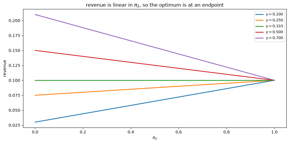
Plot the seller’s revenue against \(\pi_2 \in [0, 1]\) for several values of \(\gamma\), and confirm that it is linear.
Conclude that the optimum is always at an endpoint, so the low type receives either full information or none.
Bergemann et al. [2018] show that the low type receives the fully informative experiment if and only if \(\gamma \leq (1 - \theta^L)/(1 - \theta^H)\).
Locate the switch point numerically by bisection and compare.
Why is the answer extremal here, when the noncongruent case in the lecture produced an interior \(\pi_1 = 4/5\)?
Solution
Here is one solution:
tL_c, tH_c = 0.9, 0.7
p2_grid = np.linspace(0, 1, 401)

fig, ax = plt.subplots()
for gamma in [0.1, 0.25, 1/3, 0.5, 0.7]:
    r = np.array([two_type_revenue(1.0, p2, tL_c, tH_c, gamma) for p2 in p2_grid])
    dev = np.abs(r - np.interp(p2_grid, [0, 1], [r[0], r[-1]])).max()
    ax.plot(p2_grid, r, lw=2, label=rf'$\gamma = {gamma:.3f}$')
    print(f'gamma = {gamma:.3f}:  revenue at pi2=0 is {r[0]:.5f}, '
          f'at pi2=1 is {r[-1]:.5f},  deviation from linear {dev:.1e}')
ax.set(xlabel=r'$\pi_2$', ylabel='revenue',
       title='revenue is linear in $\pi_2$, so the optimum is at an endpoint')
ax.legend(fontsize=9)
fig.tight_layout()
plt.show()
gamma = 0.100:  revenue at pi2=0 is 0.03000, at pi2=1 is 0.10000,  deviation from linear 8.3e-17
gamma = 0.250:  revenue at pi2=0 is 0.07500, at pi2=1 is 0.10000,  deviation from linear 8.3e-17
gamma = 0.333:  revenue at pi2=0 is 0.10000, at pi2=1 is 0.10000,  deviation from linear 9.7e-17
gamma = 0.500:  revenue at pi2=0 is 0.15000, at pi2=1 is 0.10000,  deviation from linear 9.7e-17
gamma = 0.700:  revenue at pi2=0 is 0.21000, at pi2=1 is 0.10000,  deviation from linear 1.1e-16
lo, hi = 0.0, 1.0
for _ in range(60):
    mid = (lo + hi) / 2
    if two_type_revenue(1, 1, tL_c, tH_c, mid) >= two_type_revenue(1, 0, tL_c, tH_c, mid):
        lo = mid
    else:
        hi = mid

print(f'numerical switch point            gamma = {lo:.6f}')
print(f'(1 - theta_L) / (1 - theta_H)           = {(1 - tL_c) / (1 - tH_c):.6f}')
numerical switch point            gamma = 0.333333
(1 - theta_L) / (1 - theta_H)           = 0.333333
Revenue is linear in \(\pi_2\) to machine precision, so the optimum is always at \(\pi_2 \in \{0, 1\}\), and the switch occurs exactly at \(\gamma = 1/3\) as predicted.
The reason for the extremal answer is that with congruent beliefs both types would choose \(a_1\) anyway, so the only question is how much the seller reveals about \(\omega_2\).
Both types then value the experiment through the same term \((1 - \theta)\pi_2 u_2\), which is why the objective and constraints are linear in the single variable \(\pi_2\) and why the no-haggling logic of Riley and Zeckhauser [1983] applies.
With noncongruent beliefs the two types take different actions on their own, the kink in the value function lies between them, and the seller can position an experiment so that it is worth much to one type and little to the other.
That possibility is what makes an interior distortion optimal.
Exercise 36.2
Corollary 1 of Bergemann et al. [2018] states that the optimal menu contains a single item whenever both virtual values (36.16) are strictly increasing, and that for uniformly distributed types this holds irrespective of the payoffs \((u_1, u_2)\).
Verify this by solving the seller’s problem with uniform types for several asymmetric payoff pairs, for instance \((u_1, u_2) \in \{(1, 1), (2, 1), (1, 3), (5, 1)\}\).
For each case report \(\theta^*\), the interval of types served, and the price.
Confirm that the fully informative experiment is always the item offered, as Proposition 36.1 requires.
Solution
Here is one solution:
print(f'{"u1":>4s}{"u2":>4s}{"theta*":>9s}{"q offered":>12s}'
      f'{"types served":>22s}{"price":>9s}')
for u1_, u2_ in [(1, 1), (2, 1), (1, 3), (5, 1)]:
    q_a, _ = solve_menu(theta_g, np.ones(N), u1_, u2_)
    star = u2_ / (u1_ + u2_)
    served = [it for it in menu_items(theta_g, q_a, u1_, u2_) if it[3] > 1e-9]
    v, lo, hi, p = served[0]
    print(f'{u1_:4d}{u2_:4d}{star:9.4f}{v:12.4f}'
          f'{f"[{lo:.3f}, {hi:.3f}]":>22s}{p:9.4f}')
    assert abs(v - (u1_ - u2_)) < 1e-3          # the item is fully informative
print('\nevery menu contains exactly one informative item, '
      'and it is the fully informative one')
  u1  u2   theta*   q offered          types served    price
   1   1   0.5000     -0.0000        [0.250, 0.750]   0.2500
   2   1   0.3333      1.0000        [0.167, 0.666]   0.3340
   1   3   0.7500     -2.0000        [0.375, 0.875]   0.3750
   5   1   0.1667      4.0000        [0.084, 0.584]   0.4200

every menu contains exactly one informative item, and it is the fully informative one
The virtual values for a uniform density are \(\phi^-(\theta) = 2\theta\) and \(\phi^+(\theta) = 2\theta - 1\) whatever the payoffs, because \(u_1\) and \(u_2\) enter the seller’s problem only through \(d = u_1 - u_2\) and the bounds on \(q\), not through \(f\) or \(F\).
Both are strictly increasing, so no ironing is needed and a single item is optimal.
The payoffs do move \(\theta^*\) and hence which types are served and at what price, but they never make versioning worthwhile under a uniform density.
Exercise 36.3
This exercise connects the lecture back to Blackwell’s Theorem on Comparing Experiments.
Blackwell’s theorem says that if \(E'\) is a garbling of \(E\) then every decision maker weakly prefers \(E\).
Draw many random pairs of binary experiments with \(\pi_1 + \pi_2 \geq 1\).
For each pair, use
garblingto decide whether one is a garbling of the other, and separately compute whether one dominates the other in value at every type on a fine grid.Confirm that garbling implies unanimous preference, and report what fraction of random pairs Blackwell’s order fails to rank.
Among the unranked pairs, verify that some types prefer one experiment and some the other.
Solution
Here is one solution:
rng = np.random.default_rng(0)
grid_t = np.linspace(0.001, 0.999, 999)

n_pairs, n_garble, n_unranked, n_disagree, violations = 4000, 0, 0, 0, 0
for _ in range(n_pairs):
    (a1, a2), (b1, b2) = rng.uniform(0, 1, 2), rng.uniform(0, 1, 2)
    if a1 + a2 < 1 or b1 + b2 < 1:
        continue
    Ea, Eb = experiment(a1, a2), experiment(b1, b2)
    va, vb = value(a1, a2, grid_t), value(b1, b2, grid_t)

    a_garbles_b = garbling(Ea, Eb) is not None      # Eb is a garbling of Ea
    b_garbles_a = garbling(Eb, Ea) is not None
    a_dominates = np.all(va >= vb - 1e-9)
    b_dominates = np.all(vb >= va - 1e-9)

    if a_garbles_b:
        n_garble += 1
        if not a_dominates:
            violations += 1
    if b_garbles_a:
        n_garble += 1
        if not b_dominates:
            violations += 1
    if not (a_garbles_b or b_garbles_a):
        n_unranked += 1
        if not (a_dominates or b_dominates):
            n_disagree += 1

print(f'garbling relations found        {n_garble}')
print(f'violations of Blackwell         {violations}')
print(f'pairs unranked by Blackwell     {n_unranked}')
print(f'  of which types disagree       {n_disagree} '
      f'({100 * n_disagree / n_unranked:.1f}%)')
garbling relations found        674
violations of Blackwell         0
pairs unranked by Blackwell     318
  of which types disagree       317 (99.7%)
Blackwell’s theorem is never violated: whenever one experiment garbles into the other, every type prefers the garbling source.
A large share of random pairs is left unranked, and for essentially all of those the types genuinely disagree, with some preferring one experiment and some the other.
That unranked region is exactly the room the data seller needs.
If Blackwell’s order were complete, every buyer would agree on the ranking of all information products, the seller’s problem would collapse to standard nonlinear pricing over a single quality index, and the horizontal screening described in this lecture would be impossible.