37. Market Diffusion with Two-Sided Learning#
37.1. Overview#
In The Design and Price of Information a monopolist owned information and sold it.
This lecture studies a market in which nobody sells information and everybody produces it.
We follow Bergemann and Välimäki [1997], who study a duopoly in which an established firm competes on price with a firm selling a new product of unknown quality.
Buyers learn what the new product is worth only by using it, and the aggregate record of their experience is public.
So every purchase of the new product is simultaneously a consumption decision and an experiment, and its informational value spills over to everyone.
Both sides of the market learn from the same public record, which is what “two-sided learning” means here: buyers and sellers hold identical beliefs at every date, and no asymmetric information ever arises.
Three results organize the lecture.
First, both firms want more information, but only the new firm’s sales produce it.
That asymmetry softens price competition: the established firm prices less aggressively than it would in a one-shot game, and the entrant captures a larger market share early on.
Second, equilibrium experimentation is excessive when beliefs are pessimistic and insufficient when they are optimistic, with a single crossing in between.
Third, the diffusion path of a successful new product is S-shaped, matching a long empirical tradition, and the inflection occurs at a belief we can pin down exactly.
Note
The connection to the rest of this section runs through the value of information.
Blackwell’s Theorem on Comparing Experiments shows that a decision maker benefits from a more informative experiment exactly when the value of the decision problem is convex in the belief, since a more informative experiment spreads the posterior in the convex order.
Here beliefs are a martingale and experimentation controls how fast they spread, so each firm’s gain from experimentation is governed by the convexity of its value function.
The belief itself is driven by a log-likelihood-ratio process of the kind studied in Likelihood Ratio Processes, now run in continuous time.
Let’s start with imports.
import matplotlib.pyplot as plt
import numpy as np

plt.rcParams['figure.figsize'] = (10, 5)
np.set_printoptions(precision=4, suppress=True)
37.2. The market#
Buyers are distributed uniformly on \([0, 1]\) and each demands one unit per instant.
The established product delivers value
to buyer \(n\), and the new product delivers
The parameter \(h > 0\) measures horizontal differentiation, so buyers near \(n = 0\) are naturally drawn to the new product and buyers near \(n = 1\) to the established one.
This is the standard Hotelling structure, with one twist: the vertical quality \(\mu\) of the new product is unknown and can take one of two values,
The inner inequalities say the new product may be better or worse than the established one.
The outer inequalities say that under full information both firms would retain a positive share of the market, so the innovation is not drastic.
Marginal cost is zero for both firms.
If the new firm serves the buyers in \([0, n]\), the average flow value delivered by each product is
so total surplus per unit of time is \(n \bar\mu(n) + (1-n)\bar s(n)\).
Writing \(\mu(\alpha)\) for the expected quality under belief \(\alpha = \Pr[\mu = \mu_H]\), a little algebra puts the flow surplus in a convenient quadratic form,
class Market:
    """The duopoly of Bergemann and Valimaki (1997)."""

    def __init__(self, s=4.0, h=1.0, mu_L=3.1, mu_H=4.9, sigma=1.0):
        self.s, self.h = s, h
        self.mu_L, self.mu_H, self.sigma = mu_L, mu_H, sigma
        assert 0 < s - h < mu_L < s < mu_H < s + h, 'condition (4) fails'

    def mu(self, a):
        """Expected quality of the new product under belief a."""
        return (1 - a) * self.mu_L + a * self.mu_H

    def flow_surplus(self, n, a):
        return (self.s + self.h / 2 + n * (self.mu(a) - self.s + self.h)
                - n ** 2 * self.h)
37.3. Two-sided learning#
A buyer’s individual experience is a noisy draw on \(\mu\), and since each buyer has measure zero, only the aggregate record matters.
When a fraction \(n\) of buyers uses the new product, the cumulative market outcome \(X\) evolves as
so both the drift and the variance scale with the size of the experiment \(n\).
Everyone observes \(X\), so beliefs stay common.
Since \(\mu\) takes only two values, the belief \(\alpha_t = \Pr[\mu = \mu_H \mid \mathcal F_t]\) is a sufficient statistic.
Proposition 37.1 (Posterior belief)
The belief \(\alpha_t\) is a martingale with zero drift and instantaneous variance
This is the standard filtering result for a two-point prior observed through a diffusion; see Liptser and Shiryaev [1977].
Two features of (37.7) drive everything.
The variance is linear in \(n\), so information arrives in proportion to the size of the experiment, and only the new firm’s sales generate it.
The variance is proportional to \(\alpha^2(1-\alpha)^2\), so learning is fastest when beliefs are most diffuse and grinds to a halt as \(\alpha\) approaches \(0\) or \(1\).
37.3.1. Learning as a likelihood ratio process#
It is worth seeing where (37.7) comes from, because the mechanism is the one studied in Likelihood Ratio Processes, transplanted to continuous time.
Over a short interval of length \(\Delta\) the increment \(\Delta X\) is normal with mean \(n \mu \Delta\) and variance \(\sigma^2 n \Delta\) under either hypothesis, so the increment to the log likelihood ratio is
Beliefs then follow from Bayes’ rule in its log-odds form, exactly as in the discrete time lectures,
We implement (37.8) and (37.9) directly, which gives an exact Bayesian update at each step rather than a discretization of a stochastic differential equation.
def simulate_beliefs(mkt, alpha0, T, dt, mu_true, rng, policy):
    """Simulate beliefs by exact Bayesian updating of the log odds.

    `mu_true` holds the true quality for each path, so the paths run in parallel.
    Returns an array of shape (number of paths, number of steps + 1).
    """
    mu_true = np.atleast_1d(np.asarray(mu_true, dtype=float))
    M, steps = len(mu_true), int(T / dt)
    a = np.empty((M, steps + 1))
    a[:, 0] = alpha0
    ell = np.full(M, np.log(alpha0 / (1 - alpha0)))
    dmu, half = mkt.mu_H - mkt.mu_L, (mkt.mu_H ** 2 - mkt.mu_L ** 2) / 2
    for k in range(steps):
        n = policy(a[:, k])
        dX = n * mu_true * dt + mkt.sigma * np.sqrt(n * dt) * rng.standard_normal(M)
        ell += (dmu * dX - n * dt * half) / mkt.sigma ** 2
        a[:, k + 1] = 1 / (1 + np.exp(-ell))
    return a
Before using it, we check Proposition 37.1 by Monte Carlo.
def Sigma2(mkt, a):
    return (a * (1 - a) * (mkt.mu_H - mkt.mu_L) / mkt.sigma) ** 2


mkt = Market()
rng = np.random.default_rng(0)
dt, n_draw = 1e-4, 400_000

print(f'{"alpha":>7s}{"simulated var/dt":>19s}{"formula n*Sigma^2":>20s}'
      f'{"mean/dt (s.e.)":>22s}')
for a0 in [0.2, 0.5, 0.8]:
    n = 0.5                                   # hold the experiment size fixed
    ell0 = np.log(a0 / (1 - a0))
    steps = []
    for mu_true, w in [(mkt.mu_H, a0), (mkt.mu_L, 1 - a0)]:
        k = int(n_draw * w)
        dX = n * mu_true * dt + mkt.sigma * np.sqrt(n * dt) * rng.standard_normal(k)
        ell = ell0 + ((mkt.mu_H - mkt.mu_L) * dX
                      - n * dt * (mkt.mu_H ** 2 - mkt.mu_L ** 2) / 2) / mkt.sigma ** 2
        steps.append(1 / (1 + np.exp(-ell)) - a0)
    d = np.concatenate(steps)
    se = d.std() / np.sqrt(len(d)) / dt
    print(f'{a0:7.2f}{d.var() / dt:19.6f}{n * Sigma2(mkt, a0):20.6f}'
          f'{d.mean() / dt:14.4f} ({se:.3f})')
  alpha   simulated var/dt   formula n*Sigma^2        mean/dt (s.e.)
   0.20           0.041586            0.041472        0.0034 (0.032)
   0.50           0.101145            0.101250        0.0606 (0.050)
   0.80           0.041428            0.041472        0.0096 (0.032)
The simulated variance matches (37.7), and the mean increment is indistinguishable from zero, confirming that beliefs form a martingale.
37.4. Efficient experimentation#
A planner choosing \(n(\alpha)\) trades current surplus against the information that sales generate.
Bergemann and Välimäki [1997] avoid the nonlinear differential equations that discounting would produce by working with the undiscounted limit, using the strong long-run average criterion of Dutta [1991].
The optimal policies in this limit are the limits of the discounted policies as the discount rate goes to zero, so the intertemporal tradeoff survives.
The Bellman equation becomes
where \(v(\alpha)\) is the long-run average attainable under full information and the last term is the value of information: the size of the experiment \(n\) times the speed of learning \(\Sigma^2\) times the shadow price \(V''\).
Because the belief is a martingale, no first-derivative term appears.
Since \(\mu\) is eventually learned, \(v\) is just the linear interpolation of the two full-information values,
The clever step is that the maximized bracket in (37.10) equals zero, so we may divide through by \(n\) without changing the maximizer.
Doing so removes \(V''\) from the first-order condition entirely and leaves
whose first-order condition gives the efficient policy in closed form.
Proposition 37.2 (Efficient experimentation)
The efficient market share of the new product is
The myopic planner, who ignores the informational value of sales, instead sets \(m^*(\alpha) = \arg\max_n F(n,\alpha)\).
def v_social(mkt, a):
    s, h = mkt.s, mkt.h
    return ((s + mkt.mu(a) + 1.5 * h) / 2
            + (1 - a) * (mkt.mu_L - s) ** 2 / (4 * h)
            + a * (mkt.mu_H - s) ** 2 / (4 * h))


def n_star(mkt, a):
    """Efficient share, equation (nstar)."""
    return np.sqrt((v_social(mkt, a) - mkt.s - mkt.h / 2) / mkt.h)


def m_star(mkt, a):
    """Myopically efficient share."""
    return (mkt.mu(a) - mkt.s + mkt.h) / (2 * mkt.h)
At \(\alpha \in \{0, 1\}\) there is nothing left to learn, so the two must agree, and they do.
for a, mu_i in [(0.0, mkt.mu_L), (1.0, mkt.mu_H)]:
    direct = (mu_i - mkt.s + mkt.h) / (2 * mkt.h)
    print(f'alpha = {a}:  n* = {n_star(mkt, a):.6f}   '
          f'full-information share = {direct:.6f}')

A = np.linspace(1e-6, 1 - 1e-6, 4001)          # full grid, for plotting
A_int = np.linspace(0.05, 0.95, 1801)          # strictly interior grid

gap_myopic = n_star(mkt, A_int) - m_star(mkt, A_int)
print(f'\nn*(alpha) - m*(alpha) on [0.05, 0.95]:  '
      f'min {gap_myopic.min():.5f},  at alpha = 0.5 it is '
      f'{float(n_star(mkt, 0.5) - m_star(mkt, 0.5)):.5f}')
alpha = 0.0:  n* = 0.050000   full-information share = 0.050000
alpha = 1.0:  n* = 0.950000   full-information share = 0.950000

n*(alpha) - m*(alpha) on [0.05, 0.95]:  min 0.02101,  at alpha = 0.5 it is 0.17268
The planner always experiments more than the myopic benchmark, which is the intertemporal value of information showing up as extra sales of the new product.
37.5. Equilibrium#
Now let the two firms set prices \(p_1\) and \(p_2\) and let buyers choose.
The marginal buyer \(n\) is indifferent when \(s + nh - p_1 = \mu(\alpha) + (1-n)h - p_2\), which pins the market share to prices.
Each firm solves a dynamic program in which its own value of information appears, and the same divide-by-\(n\) trick removes the second derivatives from the first-order conditions.
Proposition 37.3 (Equilibrium)
There is a unique Markov-perfect equilibrium, with
and market share of the new firm
where \(v_i(\alpha)\) is firm \(i\)’s full-information long-run average revenue.
def v1(mkt, a):
    s, h = mkt.s, mkt.h
    return ((1 - a) * ((s - mkt.mu_L) / 3 + h) ** 2 / (2 * h)
            + a * ((s - mkt.mu_H) / 3 + h) ** 2 / (2 * h))


def v2(mkt, a):
    s, h = mkt.s, mkt.h
    return ((1 - a) * ((mkt.mu_L - s) / 3 + h) ** 2 / (2 * h)
            + a * ((mkt.mu_H - s) / 3 + h) ** 2 / (2 * h))


def n_eq(mkt, a):
    return np.sqrt(v2(mkt, a) / (2 * mkt.h))


def p1(mkt, a):
    return 2 / 3 * (mkt.s - mkt.mu(a)) + np.sqrt(2 * mkt.h * v2(mkt, a))


def p2(mkt, a):
    return (mkt.mu(a) - mkt.s) / 3 + mkt.h


def p1_myopic(mkt, a):
    return (mkt.s - mkt.mu(a)) / 3 + mkt.h


def n_myopic(mkt, a):
    return ((mkt.mu(a) - mkt.s) / 3 + mkt.h) / (2 * mkt.h)
Comparing the dynamic equilibrium with the static one played period by period reveals the asymmetry at the heart of the paper.
print('comparing the dynamic equilibrium with the static one, on [0.05, 0.95]')
print(f'  max |p2 - p2_myopic|   {np.abs(p2(mkt, A_int) - p2(mkt, A_int)).max():.2e}')
print(f'  min (p1 - p1_myopic)   {(p1(mkt, A_int) - p1_myopic(mkt, A_int)).min():.5f}')
print(f'  min (n_eq - n_myopic)  {(n_eq(mkt, A_int) - n_myopic(mkt, A_int)).min():.5f}')
comparing the dynamic equilibrium with the static one, on [0.05, 0.95]
  max |p2 - p2_myopic|   0.00e+00
  min (p1 - p1_myopic)   0.00671
  min (n_eq - n_myopic)  0.00336
The new firm’s price is exactly its myopic price, a knife-edge consequence of the linear preference structure and the absence of discounting.
The established firm charges more than it would in a one-shot game, and so concedes market share.
That is the striking result: the incumbent softens competition, not out of weakness, but because the entrant’s sales are the only source of information and the incumbent wants the information.
37.5.1. Who values information more?#
The Bellman equations imply that each firm’s value of information equals the gap between its expected full-information revenue and its current revenue.
voi_1 = v1(mkt, A) - (1 - n_eq(mkt, A)) * p1(mkt, A)
voi_2 = v2(mkt, A) - n_eq(mkt, A) * p2(mkt, A)

print(f'established firm, minimum value of information  {voi_1.min():.3e}')
print(f'new firm, minimum value of information          {voi_2.min():.3e}')
print(f'ratio voi_1 / voi_2:  min {np.min(voi_1 / voi_2):.6f}, '
      f'max {np.max(voi_1 / voi_2):.6f}')
established firm, minimum value of information  1.800e-07
new firm, minimum value of information          9.000e-08
ratio voi_1 / voi_2:  min 2.000000, max 2.000000
Both are positive, so both value functions are convex in the belief.
That is the Blackwell’s Theorem on Comparing Experiments logic at work: beliefs are a martingale, more experimentation spreads them further, and a firm with a convex value function gains from the spread.
More surprisingly, the ratio is exactly \(2\) at every belief.
The established firm values information twice as much as the entrant, because in equilibrium it is the incumbent that has given up current revenue relative to what it would earn once uncertainty is resolved.
37.6. Too much experimentation, then too little#
We can now compare the equilibrium share with the efficient one.
gap = n_star(mkt, A) - n_eq(mkt, A)
cross = A[np.argmin(np.abs(gap))]

fig, axes = plt.subplots(1, 2, figsize=(12, 4.2))
axes[0].plot(A, n_star(mkt, A), lw=2, label=r'efficient $n^*(\alpha)$')
axes[0].plot(A, n_eq(mkt, A), lw=2, label=r'equilibrium $n(\alpha)$')
axes[0].plot(A, m_star(mkt, A), lw=1.5, ls='--', color='0.5',
             label=r'myopic planner $m^*(\alpha)$')
axes[0].set(xlabel=r'$\alpha$', ylabel='market share of the new firm',
            title='experimentation policies')
axes[0].legend(fontsize=9)

axes[1].plot(A, gap, lw=2, color='C3')
axes[1].axhline(0, color='0.3', lw=1)
axes[1].axvline(cross, color='0.6', ls=':', lw=1.5)
axes[1].fill_between(A, gap, 0, where=gap < 0, alpha=0.15, color='C3')
axes[1].fill_between(A, gap, 0, where=gap > 0, alpha=0.15, color='C0')
axes[1].annotate('equilibrium\nexperiments too much', (0.05, gap.min() / 2),
                 fontsize=9)
axes[1].annotate('too little', (0.75, gap.max() / 2), fontsize=9)
axes[1].set(xlabel=r'$\alpha$', ylabel=r'$n^*(\alpha) - n(\alpha)$',
            title=f'single crossing at ' + rf'$\alpha = {cross:.3f}$')
fig.tight_layout()
plt.show()

print(f'gap is monotone increasing: {np.all(np.diff(gap) > 0)}')
print(f'number of sign changes:     {int(np.sum(np.diff(np.sign(gap)) != 0))}')
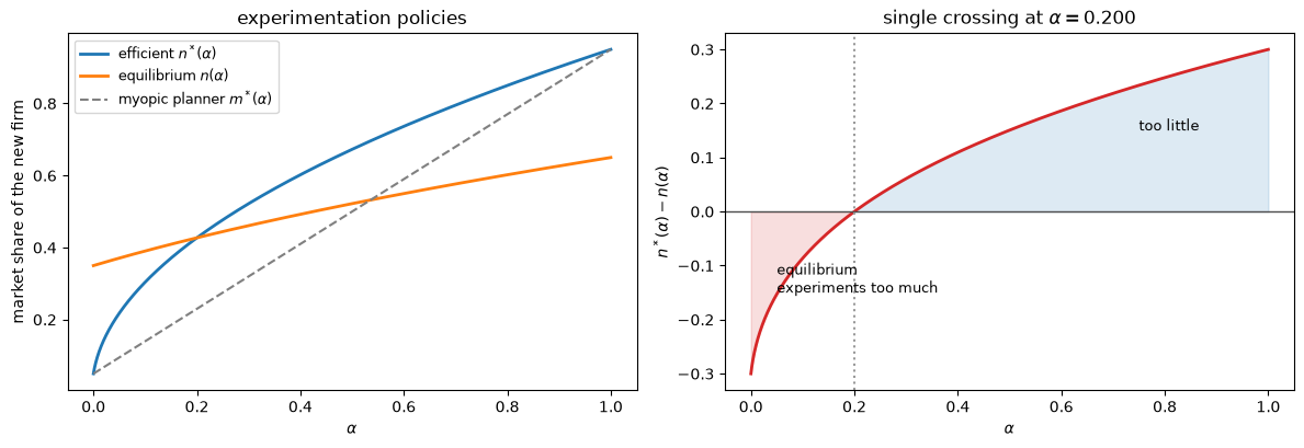
Fig. 37.1 Equilibrium versus efficient experimentation#
gap is monotone increasing: True
number of sign changes:     1
The intuition is about who has to cut price to gain a buyer.
At pessimistic beliefs the entrant is small, so attracting one more buyer costs it little in inframarginal revenue, while the incumbent is large and unwilling to defend its share by cutting price on everyone.
The entrant therefore expands aggressively and the market over-experiments.
At optimistic beliefs the positions are reversed, the incumbent fights harder, and experimentation falls short of the efficient level.
37.7. Diffusion over time#
So far everything is a function of the state \(\alpha\).
To follow a product over calendar time we need the law of motion of the belief when the product really is good.
Conditional on \(\mu = \mu_H\), the belief acquires an upward drift, since the data are generated by \(\mu_H\) while the market still puts weight \(1 - \alpha\) on \(\mu_L\),
Stripping out the noise gives a deterministic path for the mean belief.
def mean_belief_path(mkt, alpha0, T, dt, policy):
    """Deterministic path of the mean posterior when mu = mu_H."""
    steps = int(T / dt)
    a = np.empty(steps + 1)
    a[0] = alpha0
    dmu2 = (mkt.mu_H - mkt.mu_L) ** 2 / mkt.sigma ** 2
    for k in range(steps):
        drift = policy(a[k]) * dmu2 * a[k] * (1 - a[k]) ** 2
        a[k + 1] = min(max(a[k] + drift * dt, 1e-12), 1 - 1e-12)
    return a
Proposition 37.4 (S-shaped diffusion)
Conditional on the product being good, the mean market share \(\hat n(t)\) is increasing over time.
Its rate of increase is itself increasing while \(\hat\alpha(t) \leq 1/3\) and decreasing thereafter.
The composition of two forces produces the S.
Learning accelerates as beliefs move away from zero, which speeds up the growth of the entrant’s share; but the equilibrium share \(n(\alpha)\) is concave, so further belief improvements translate into ever smaller share gains.
T, dt, alpha0 = 8.0, 1e-3, 0.03
policy = lambda a: n_eq(mkt, a)

a_mean = mean_belief_path(mkt, alpha0, T, dt, policy)
t_grid = np.linspace(0, T, len(a_mean))

rng = np.random.default_rng(12)
paths = simulate_beliefs(mkt, alpha0, T, dt, np.full(6, mkt.mu_H), rng, policy)

fig, axes = plt.subplots(1, 2, figsize=(12, 4.2))
for pth in paths:
    axes[0].plot(t_grid, pth, lw=0.7, alpha=0.55, color='C0')
axes[0].plot(t_grid, a_mean, lw=2.5, color='C3', label='mean path')
axes[0].axhline(1 / 3, color='0.5', ls=':', lw=1.5)
axes[0].set(xlabel='time', ylabel=r'$\alpha(t)$', title='beliefs')
axes[0].legend(fontsize=9)

for pth in paths:
    axes[1].plot(t_grid, n_eq(mkt, pth), lw=0.7, alpha=0.55, color='C0')
axes[1].plot(t_grid, n_eq(mkt, a_mean), lw=2.5, color='C3', label='mean path')
axes[1].set(xlabel='time', ylabel=r'$n(t)$',
            title='market share of the new firm')
axes[1].legend(fontsize=9)
fig.tight_layout()
plt.show()
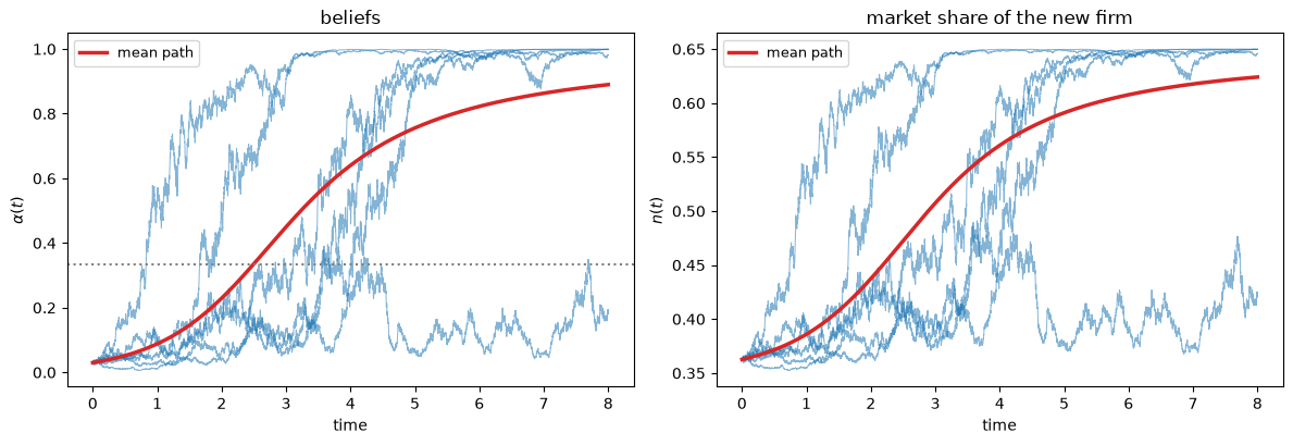
Fig. 37.2 The S-shaped diffusion path of a successful new product#
The inflection point is exactly where Proposition 37.4 says it is.
n_mean = n_eq(mkt, a_mean)
growth = np.gradient(n_mean, t_grid)
k = np.argmax(growth)
print(f'share grows fastest at t = {t_grid[k]:.3f}, '
      f'where alpha = {a_mean[k]:.4f}   (theory: 1/3)')

drift = policy(A) * (mkt.mu_H - mkt.mu_L) ** 2 * A * (1 - A) ** 2
print(f'belief drift peaks at alpha = {A[np.argmax(drift)]:.4f}   '
      f'(theory: between 1/3 and 2/3)')
share grows fastest at t = 2.490, where alpha = 0.3334   (theory: 1/3)
belief drift peaks at alpha = 0.3830   (theory: between 1/3 and 2/3)
Prices move in step with shares.
fig, ax = plt.subplots()
for pth in paths:
    ax.plot(t_grid, p1(mkt, pth), lw=0.7, alpha=0.5, color='C0')
    ax.plot(t_grid, p2(mkt, pth), lw=0.7, alpha=0.5, color='C1')
ax.plot(t_grid, p1(mkt, a_mean), lw=2.5, color='C0',
        label=r'$p_1$, established firm')
ax.plot(t_grid, p2(mkt, a_mean), lw=2.5, color='C1', label=r'$p_2$, new firm')
ax.set(xlabel='time', ylabel='price',
       title='the incumbent retreats as the entrant is vindicated')
ax.legend()
fig.tight_layout()
plt.show()
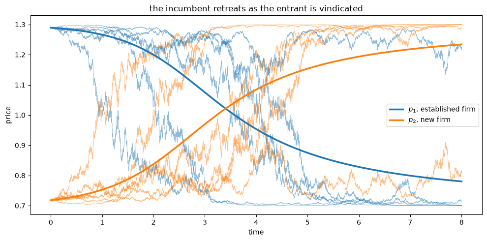
Fig. 37.3 Price paths of the two firms#
37.8. Martingale properties#
Bergemann and Välimäki [1997] characterize the equilibrium objects probabilistically: the entrant’s price is a martingale, the incumbent’s price and the entrant’s share are supermartingales, and both revenues are submartingales.
Because \(\alpha\) is a martingale, each of these follows from the shape of the corresponding function of \(\alpha\), and we can check them all by simulation.
rng = np.random.default_rng(3)
a0, M = 0.5, 20_000

# draw the true quality from the prior, one value per path
mu_true = np.where(rng.random(M) < a0, mkt.mu_H, mkt.mu_L)
ends = simulate_beliefs(mkt, a0, 4.0, 2e-3, mu_true, rng, policy)[:, -1]

rows = [
    ('belief', a0, ends.mean(), 'martingale'),
    ('share of new firm', n_eq(mkt, a0), n_eq(mkt, ends).mean(), 'supermartingale'),
    ('price of new firm', p2(mkt, a0), p2(mkt, ends).mean(), 'martingale'),
    ('price of incumbent', p1(mkt, a0), p1(mkt, ends).mean(), 'supermartingale'),
    ('revenue of incumbent', (1 - n_eq(mkt, a0)) * p1(mkt, a0),
     ((1 - n_eq(mkt, ends)) * p1(mkt, ends)).mean(), 'submartingale'),
    ('revenue of new firm', n_eq(mkt, a0) * p2(mkt, a0),
     (n_eq(mkt, ends) * p2(mkt, ends)).mean(), 'submartingale')]

print(f'{"":24s}{"t = 0":>10s}{"E[t = 4]":>11s}{"change":>10s}   prediction')
for name, x0, xT, pred in rows:
    print(f'{name:24s}{x0:10.4f}{xT:11.4f}{xT - x0:+10.4f}   {pred}')
                             t = 0   E[t = 4]    change   prediction
belief                      0.5000     0.5010   +0.0010   martingale
share of new firm           0.5220     0.5072   -0.0148   supermartingale
price of new firm           1.0000     1.0006   +0.0006   martingale
price of incumbent          1.0440     1.0132   -0.0308   supermartingale
revenue of incumbent        0.4990     0.5310   +0.0320   submartingale
revenue of new firm         0.5220     0.5389   +0.0168   submartingale
Every sign comes out as predicted.
The entrant’s expected share falls over time even though its share rises conditional on the product being good, because the early aggression reflects the value of information rather than confidence in the product.
Both firms expect to earn more later, which is the sense in which they sacrifice current profit to buy information.
37.9. Concluding remarks#
Two lectures in this section now feature information whose value is entirely instrumental.
In The Design and Price of Information a seller designs and prices experiments, and the interesting economics comes from the fact that Blackwell’s order is incomplete.
Here nobody prices information at all, and the interesting economics comes from the fact that only one firm’s sales produce it.
Both rest on the same foundation from Blackwell’s Theorem on Comparing Experiments: information is valuable to a decision maker exactly to the extent that the value of the decision problem is convex in the belief.
The distinctive lesson of Bergemann and Välimäki [1997] is that this convexity is shared by competitors.
Because both firms would rather face a market that has sorted out the quality of the new product, uncertainty about vertical quality relaxes price competition much as deterministic differentiation does in Shaked and Sutton [1982].
That is why the incumbent lets the entrant in cheaply at first and why a successful product diffuses along an S-shaped path.
The continuous-time technique used here, and in particular the device of taking the undiscounted limit to keep the Bellman equations tractable, comes from Bolton and Harris [1999], who were the first to study strategic experimentation in continuous time.
A companion paper, Bergemann and Välimäki [2000], studies the same duopoly with a continuum of identical consumers.
Homogeneity there rules out market sharing, so the horizontal differentiation that generates the diffusion path in this lecture is absent and the analysis concentrates instead on how informational externalities affect market efficiency.
37.10. Exercises#
Exercise 37.1
Condition (37.3) requires \(|\mu_i - s| < h\) for both quality levels.
Show algebraically that this confines the full-information equilibrium share of the new firm to the interval \((1/3, 2/3)\), and hence that \(n(\alpha) \in (1/3, 2/3)\) for every belief.
Verify this numerically for several admissible \((\mu_L, \mu_H)\) pairs.
Bergemann and Välimäki [1997] draw their diffusion figures with \(s = 4\), \(h = 1\), \(\mu_L = 2\) and \(\mu_H = 6\).
Check whether these satisfy (37.3), compute the equilibrium shares at \(\alpha \in \{0, 1\}\), and compute the myopically efficient share \(m^*\) at each quality level.
What goes wrong, and which of the lecture’s results still hold?
Solution
Here is one solution:
Under full information with quality \(\mu_i\) the equilibrium share is \(n_i = \bigl(\tfrac13(\mu_i - s) + h\bigr)/(2h)\).
Condition (37.3) gives \(-h < \mu_i - s < h\), so \(\tfrac13(\mu_i - s) \in (-h/3, h/3)\) and therefore \(n_i \in \bigl(\tfrac{2h/3}{2h}, \tfrac{4h/3}{2h}\bigr) = (1/3, 2/3)\).
Since \(n(\alpha)^2\) is a convex combination of \(n_0^2\) and \(n_1^2\), the equilibrium share lies between \(n_0\) and \(n_1\) for every \(\alpha\).
for mu_L, mu_H in [(3.1, 4.9), (3.4, 4.6), (3.9, 4.1)]:
    m_ = Market(mu_L=mu_L, mu_H=mu_H)
    lo, hi = n_eq(m_, 0.0), n_eq(m_, 1.0)
    print(f'(mu_L, mu_H) = ({mu_L}, {mu_H}):  n_eq ranges over '
          f'[{lo:.4f}, {hi:.4f}]   inside (1/3, 2/3): {1/3 < lo and hi < 2/3}')
(mu_L, mu_H) = (3.1, 4.9):  n_eq ranges over [0.3500, 0.6500]   inside (1/3, 2/3): True
(mu_L, mu_H) = (3.4, 4.6):  n_eq ranges over [0.4000, 0.6000]   inside (1/3, 2/3): True
(mu_L, mu_H) = (3.9, 4.1):  n_eq ranges over [0.4833, 0.5167]   inside (1/3, 2/3): True
class LooseMarket(Market):
    def __init__(self, **kw):                 # skip the assertion
        self.s, self.h = kw['s'], kw['h']
        self.mu_L, self.mu_H, self.sigma = kw['mu_L'], kw['mu_H'], kw.get('sigma', 1.0)


paper = LooseMarket(s=4, h=1, mu_L=2, mu_H=6)
print(f'condition (4) needs  s - h < mu_L:  {paper.s - paper.h} < {paper.mu_L}?  '
      f'{paper.s - paper.h < paper.mu_L}')
print(f'condition (4) needs  mu_H < s + h:  {paper.mu_H} < {paper.s + paper.h}?  '
      f'{paper.mu_H < paper.s + paper.h}')
print(f'\nequilibrium shares:   n(0) = {n_eq(paper, 0.0):.4f}, '
      f'n(1) = {n_eq(paper, 1.0):.4f}')
for mu_i, nm in [(paper.mu_L, 'mu_L'), (paper.mu_H, 'mu_H')]:
    print(f'myopically efficient share at {nm}: '
          f'{(mu_i - paper.s + paper.h) / (2 * paper.h):+.4f}')
condition (4) needs  s - h < mu_L:  3 < 2?  False
condition (4) needs  mu_H < s + h:  6 < 5?  False

equilibrium shares:   n(0) = 0.1667, n(1) = 0.8333
myopically efficient share at mu_L: -0.5000
myopically efficient share at mu_H: +1.5000
The paper’s figure parameters violate (37.3) at both ends.
The consequence is that the efficient allocation is at a corner: it would assign every buyer to the established product when \(\mu = \mu_L\) and every buyer to the new product when \(\mu = \mu_H\), so the interior formula (37.12) no longer applies and the efficiency comparison of Proposition 37.2 breaks down.
Everything about the equilibrium survives, because equilibrium shares remain strictly interior at \(1/6\) and \(5/6\).
That is why those parameters are fine for drawing diffusion paths, which is all the paper uses them for, and why they buy a much more dramatic S-curve than any admissible parameter set could.
Exercise 37.2
The lecture found a single belief at which equilibrium experimentation switches from excessive to insufficient.
Write a function that locates this crossing point by bisection.
Compute it as the quality spread \(\mu_H - \mu_L\) widens, holding the midpoint \(\tfrac12(\mu_L + \mu_H) = s\) fixed, and again as the horizontal differentiation parameter \(h\) varies.
Both experiments produce the same numbers whenever the ratio \((\mu_H - \mu_L)/h\) agrees.
Guess the closed form for the crossing point and check it numerically.
Does your formula survive when the quality midpoint is moved away from \(s\)?
Solution
Here is one solution:
def crossing(mkt, tol=1e-13):
    """Belief at which n*(alpha) = n(alpha), by bisection."""
    lo, hi = 1e-12, 1 - 1e-12
    f = lambda a: n_star(mkt, a) - n_eq(mkt, a)
    if f(lo) > 0 or f(hi) < 0:
        return np.nan
    while hi - lo > tol:
        mid = (lo + hi) / 2
        lo, hi = (mid, hi) if f(mid) < 0 else (lo, mid)
    return (lo + hi) / 2


print('widening the quality spread, midpoint fixed at s = 4, h = 1')
for spread in [0.4, 0.8, 1.2, 1.6, 1.9]:
    m_ = Market(s=4, h=1, mu_L=4 - spread / 2, mu_H=4 + spread / 2)
    print(f'   (mu_H - mu_L)/h = {spread / 1:.3f}:  crossing = {crossing(m_):.6f}')

print('\nvarying horizontal differentiation, mu = (3.4, 4.6)')
for h_ in [0.65, 0.8, 1.0, 1.5, 2.5]:
    m_ = Market(s=4, h=h_, mu_L=3.4, mu_H=4.6)
    print(f'   (mu_H - mu_L)/h = {1.2 / h_:.3f}:  crossing = {crossing(m_):.6f}')
widening the quality spread, midpoint fixed at s = 4, h = 1
   (mu_H - mu_L)/h = 0.400:  crossing = 0.433333
   (mu_H - mu_L)/h = 0.800:  crossing = 0.366667
   (mu_H - mu_L)/h = 1.200:  crossing = 0.300000
   (mu_H - mu_L)/h = 1.600:  crossing = 0.233333
   (mu_H - mu_L)/h = 1.900:  crossing = 0.183333

varying horizontal differentiation, mu = (3.4, 4.6)
   (mu_H - mu_L)/h = 1.846:  crossing = 0.192308
   (mu_H - mu_L)/h = 1.500:  crossing = 0.250000
   (mu_H - mu_L)/h = 1.200:  crossing = 0.300000
   (mu_H - mu_L)/h = 0.800:  crossing = 0.366667
   (mu_H - mu_L)/h = 0.480:  crossing = 0.420000
Sorted by the ratio \((\mu_H - \mu_L)/h\) the two tables line up, which suggests that the crossing point depends on the parameters only through that ratio.
The numbers fall on a straight line with slope \(-1/6\) through \(1/2\).
print(f'{"(mu_H-mu_L)/h":>15s}{"bisection":>12s}{"1/2 - ratio/6":>16s}{"error":>12s}')
for mu_L_, mu_H_, h_ in [(3.4, 4.6, 1.0), (3.1, 4.9, 1.0), (3.8, 4.2, 1.0),
                         (3.4, 4.6, 1.5), (3.4, 4.6, 0.8), (3.05, 4.95, 1.0)]:
    m_ = Market(s=4, h=h_, mu_L=mu_L_, mu_H=mu_H_)
    r = (mu_H_ - mu_L_) / h_
    c, pred = crossing(m_), 0.5 - r / 6
    print(f'{r:15.4f}{c:12.6f}{pred:16.6f}{c - pred:12.1e}')
  (mu_H-mu_L)/h   bisection   1/2 - ratio/6       error
         1.2000    0.300000        0.300000    -1.5e-14
         1.8000    0.200000        0.200000    -8.2e-15
         0.4000    0.433333        0.433333    -4.9e-15
         0.8000    0.366667        0.366667     1.9e-14
         1.5000    0.250000        0.250000     1.7e-14
         1.9000    0.183333        0.183333    -1.6e-14
So when the two quality levels straddle \(s\) symmetrically, the switch occurs at
which condition (37.3) keeps strictly inside \((1/6, 1/2)\), since that condition forces \(\mu_H - \mu_L < 2h\).
The region of excessive experimentation therefore shrinks as the quality spread widens relative to \(h\).
A wider spread means more is at stake in learning, and the efficient policy responds by experimenting a great deal; the equilibrium, driven by each firm’s private revenue motive, does not keep up except at the most pessimistic beliefs.
Raising \(h\) works in the opposite direction, since strongly attached buyers blunt the price instrument and let the entrant expand more freely than a planner would choose.
The symmetry is essential.
print('moving the quality midpoint away from s, with mu = (3.4, 4.6), h = 1')
for s_ in [3.9, 4.0, 4.1]:
    m_ = Market(s=s_, h=1, mu_L=3.4, mu_H=4.6)
    mid = (3.4 + 4.6) / 2
    print(f'   s = {s_}  (midpoint {mid}):  crossing = {crossing(m_):.6f}'
          f'   formula = {0.5 - 1.2 / 6:.6f}')
moving the quality midpoint away from s, with mu = (3.4, 4.6), h = 1
   s = 3.9  (midpoint 4.0):  crossing = 0.245098   formula = 0.300000
   s = 4.0  (midpoint 4.0):  crossing = 0.300000   formula = 0.300000
   s = 4.1  (midpoint 4.0):  crossing = 0.358974   formula = 0.300000
Once the midpoint no longer equals \(s\) the formula fails, so it is a knife-edge result rather than a general one.
Exercise 37.3
This exercise makes the link with Blackwell’s Theorem on Comparing Experiments precise.
In that lecture, a decision maker gains from a more informative experiment exactly when the value of the decision problem is convex in the belief, because a more informative experiment produces a mean-preserving spread of the posterior.
Here the belief is a martingale and experimentation controls the speed at which it spreads, so the same logic applies to each firm.
Plot each firm’s value of information, \(v_i(\alpha)\) minus its current equilibrium revenue, against \(\alpha\).
Confirm that both are positive everywhere in the interior and vanish at \(\alpha \in \{0, 1\}\), and explain why they must vanish there.
The value of information also equals \(\tfrac12 n(\alpha)\Sigma^2(\alpha)V_i''(\alpha)\).
Use this to recover \(V_i''(\alpha)\) and confirm that both value functions are convex.
Solution
Here is one solution:
Ai = np.linspace(0.005, 0.995, 2001)
voi_1 = v1(mkt, Ai) - (1 - n_eq(mkt, Ai)) * p1(mkt, Ai)
voi_2 = v2(mkt, Ai) - n_eq(mkt, Ai) * p2(mkt, Ai)

fig, axes = plt.subplots(1, 2, figsize=(12, 4.2))
axes[0].plot(Ai, voi_1, lw=2, label='established firm')
axes[0].plot(Ai, voi_2, lw=2, label='new firm')
axes[0].axhline(0, color='0.3', lw=1)
axes[0].set(xlabel=r'$\alpha$', ylabel='value of information',
            title='both firms gain from experimentation')
axes[0].legend(fontsize=9)

V1pp = 2 * voi_1 / (n_eq(mkt, Ai) * Sigma2(mkt, Ai))
V2pp = 2 * voi_2 / (n_eq(mkt, Ai) * Sigma2(mkt, Ai))
axes[1].plot(Ai, V1pp, lw=2, label=r"$V_1''(\alpha)$")
axes[1].plot(Ai, V2pp, lw=2, label=r"$V_2''(\alpha)$")
axes[1].set(xlabel=r'$\alpha$', yscale='log',
            title='second derivatives of the value functions')
axes[1].legend(fontsize=9)
fig.suptitle('The value of information to each firm')
fig.tight_layout()
plt.show()

print(f'minimum value of information, established firm  {voi_1.min():.3e}')
print(f'minimum value of information, new firm          {voi_2.min():.3e}')
print(f'minimum of V1\'\'  {V1pp.min():.4f}    minimum of V2\'\'  {V2pp.min():.4f}')
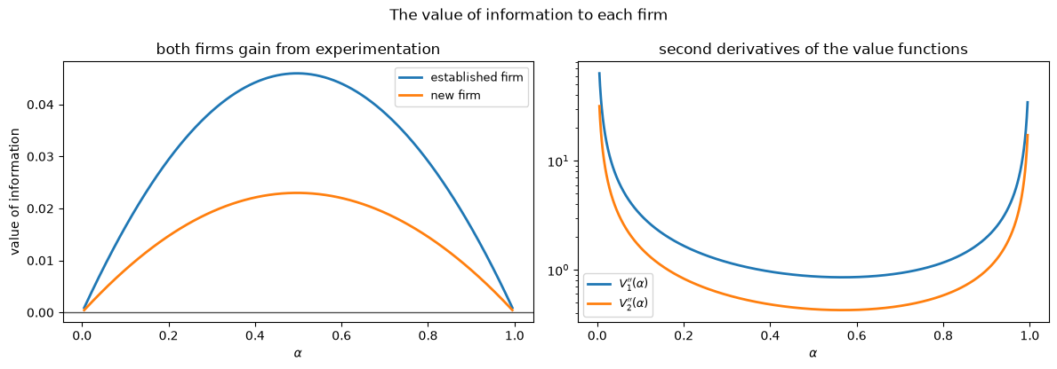
minimum value of information, established firm  8.957e-04
minimum value of information, new firm          4.479e-04
minimum of V1''  0.8531    minimum of V2''  0.4265
Both curves are strictly positive on the interior and both second derivatives are strictly positive, so both value functions are convex.
The value of information vanishes at \(\alpha \in \{0, 1\}\) for two reinforcing reasons.
There is nothing left to learn, so the equilibrium coincides with the full-information equilibrium and the revenue gap closes.
And the speed of learning \(\Sigma^2(\alpha) \propto \alpha^2(1-\alpha)^2\) vanishes as well, so even a convex value function earns nothing from an experiment that reveals nothing.
The second derivatives do not vanish at the endpoints, which is exactly the Blackwell’s Theorem on Comparing Experiments point: the willingness to pay for information stays positive, but the supply of information dries up as beliefs become degenerate.